Feb 01, 2023
The Magical Formula for Success With Microsoft Excel
Philip Wiest, Guest Blogger
Much like a magician’s grand finale trick, it’s possible to do many amazing things within one Excel formula. The formula itself may look complex, but as you’ll see, it’s not how you write the formula; it’s how you figure it out.
The Setup

This formula may look complex, but it’s the answer to a client’s wish to do a “lookup” in three directions.
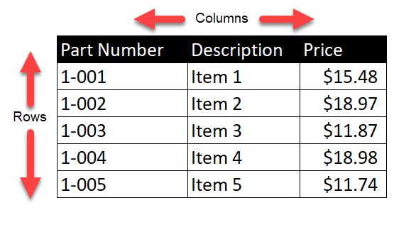
Usually one looks for “something” in two directions — at the intersection of a row and a column.
For example, in a list of Part Numbers, you’re looking for a price in Row 3 and Column 3.

The formula goes something like this:
=INDEX(TABLE, Row Number, Column Number)
=INDEX(TABLE, 3,3)
Translation: “Looking at a rectangle of cells, what’s in Row 3, Column 3?”
The Hiccup
The issue, though, is that you need to look things up in Table 1 or Table 2 — it depends!
That’s adding a third dimension to the lookup.
An Example
A government agency funds project based on 3 criteria:
- Funding Amount (a row)
- Number of people (a column)
- Funding Source (a table – either Federal or State)
Because you have multiple funding “tables,” you need the formula to take the funding “source” and select the correct lookup range.
You’ve mastered the INDEX (ARRAY MATCH(Row), MATCH(Column)) technique — one which looks at a specific array and returns whatever is at the intersection of the matching row and column.
But how do you build a formula to accommodate multiple ranges: Federal Funding OR State Funding?
The Answer
The technique to solving a complicated formula is to do it in steps – start with what you know:
=INDEX(“FEDERAL,” 3, 2)

If this matches the value at the intersection of Row 3 and Column 2, we can build on this!
We can begin to build a more flexible “INDEX MATCH MATCH” formula by replacing the static row and column values with MATCH Commands.
For example:
=INDEX(“The Range”, MATCH(2012 in the first column), MATCH(“2 People” in the top row)
If this matches the value at the intersection of the row match and the column match, we can build on this!

Then, to add a little more clarity and flexibility, we can “point” the MATCH functions to cells containing the values, like $2012.00 and “2 People.”
Notice cells G4 and G5:

We’re getting closer!
Getting the range to change — easily
The key to this “trick” is knowing how to replace a static table (named FEDERAL) buy using CHOOSE() – which takes a “choice” number (1 or 2) and returns a result (like the Federal Table or the State Table).
(Hint: use the same recipe for identifying the MATCH lookup ranges!)
CHOOSE( ) is an IF-type of formula.
It would look like this:
=CHOOSE(the choice number, “Range 1”, “Range 2”).
Whatever the option the user chooses will “drive” the output of CHOOSE to option 1, or option 2. (Table 1 or Table 2), and CHOOSE( ) what will replace any of the static ranges in your original formula!
The News About CHOOSE( )
Here’s an example of a simple CHOOSE:
=CHOOSE(“Value”, The FEDERAL Table, The STATE Table)
If the Value is “1”, then the CHOOSE function returns “The Federal Table.”
If the Value is “2”, then the CHOOSE function returns “The State Table.”

So, you can update your formula and replace each range reference with the output of a CHOOSE( ).
If the user selects 1, then the Federal ranges are inserted throughout the formula; if the user chooses 2, then the State ranges are inserted through the formula.
Let’s look at that formula! Let’s see if you can spot the “CHOOSES”!
Hint, there are three of them:
- one for the Table Lookup
- one for the Row Lookup
- one for the Column Lookup

If Cell $B$2 has a 1, it’s FEDERAL; If Cell $B$2 has a 2, it’s STATE. In this case, it’s 1 so…it’s FEDERAL!

The Technique
By going through these steps, slowly, and starting with simple static values, then gradually replacing them (in stages) with cell references having dynamic values, you’ll get your final formula faster than if you had tried to write a complex formula first.
You see, it’s never how you do the trick, it’s how the trick is done.
It’s learning the technique that makes the difference!
Ready to learn more? Check out some of SkillPath’s live virtual training programs, on-demand video training or get it all with our unlimited eLearning platform.
Philip Wiest
Guest Blogger
Philip Wiest is an expert software trainer, computer analyst and database consultant who knows both the intricacies of computer systems and the ways today’s professionals need to use these essential business tools. Using his experience in Microsoft Excel and Microsoft Office, as well as Windows and the Internet, Phil uses a special mix of tactful guidance and distilled observation so his audiences learn and retain the critical keystrokes, application combinations and creative processes that save time and simplify computer use.
Latest Articles
Article Topics
